Category: Research Blog

  • July 4 Update and Clara in Spokane

    July 4 Update and Clara in Spokane

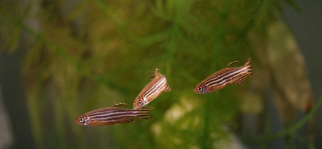
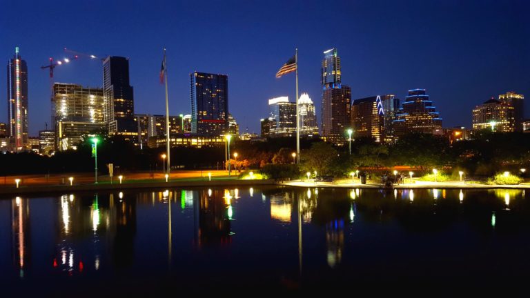
    It’s been over a month since my last update. There haven’t been any major adventures due to time and financial constraints. As I aim to write and finish my dissertation, the time for such outings decreases and thus this summer will be nicknamed “the summer of no fun.” Fun isn’t completely off the table, but the number and scope of such expeditions will be reduced compared to past years.

    City of Austin
    City of Austin

    I did have one bit of adventure in June. I traveled to Austin for the 2016 Evolution meeting where I presented some results from our behavioral simulation experiments. With our latest zebrafish experiments as inspiration, we’ve put together a program to simulate an animal’s movement in two-dimensional space as it explores its habitat and collects “food” pieces to invest in reproduction. By manipulating aspects of the environment, we can better understand how habitat usage influences risk and thus selection for or against risk-taking behaviors. Movement is determined by a neural network with weights that are heritable and represent the (quantitative) genetic basis of behavior. The simulation is very basic at this point, but already we are seeing some promising results. For example, when a “predator” is introduced represented by an probability of death in a given location, we observe behaviors evolving to avoid, or spend less time in, the high risk areas. However the degree and even direction of selection is dependent not just on the intensity of predation, but also the amount of “food” resources available.

    I had a good time at evolution, reconnecting with friends I’ve met at previous meetings, and meeting some new contacts. Rather than stay in the dorms at UT, or the expensive hotels downtown, I stayed in a hostel nearby which enhanced the social factor, as well as my budget. It turned out I wasn’t the only one with that idea and I met plenty of other conference goers at the hostel. Austin is an interesting city. It’s weird. Portland weird. I’d go as far to call it the Portland of the south. It’s a town for live music, good food, arts, and culture. There are nice bike paths and beautiful parks. But during the summer, it’s hot. Very hot. Daytime highs all week were in the mid to upper 90’s with 80-90% humidity.


    It’s the 4th of July. On many years past, I’ve taken a hike to celebrate our nation’s independence. Today I spent the day at home. We didn’t even take Clara out to see fireworks in town. It was just a lazy day. That makes up for us being out all day yesterday. We headed up to Spokane to pick up my mom from the airport and spent the afternoon at Riverside Park. After a stop at Target followed by dinner at a very great pizza place, we got home shortly before midnight. Here is some of the fun we had with Clara.

  • My Research: What I have been up to

    My Research: What I have been up to

    Last week, the fruits of my last three year’s work has finally come to fruition in the journal PLoS One. The premise is that the personality behavior we call boldness, or the bold-shy continuum, is not only heritable, but a genetically correlated multivariate trait. The research is essentially a continuation of a project Mary Oswald completed for her dissertation, however upon first submission, reviewers criticized the study for its lack of replication. So, in the Summer of 2010, she set up a second selection experiment which I took over and have been maintaining since.

    Boldness is an interesting behavior to study in animals. As a personality behavior, individuals with a particular boldness score relative to the population tend to remain that way for the long-term, and while there is some plasticity between contexts, individuals that are bold tend to remain bold, and individuals that remain shy tend to remain shy, and populations can evolve toward one end or the other based on selection pressures. Of course, the best way to really get this point across is to see some videos exhibiting just what boldness and shyness represent.

    These are Zebrafish, Danio rerio. The top tank, labelled “Nadia,” contain a wild strain, but these fish aren’t taken directly from the wild. Instead, these are the 4th generation from wild fish to be raised in captivity right here at the University of Idaho. Notice how they prefer to swim at the bottom of the water column and shy away from a human presence. Now contrast that with the bottom tank containing fish from the Scientific Hatcheries (SH) strain, which are more than 30 generations removed from captivity. They not only spend more of their time near the top of the water column, but are also un-phased by a human presence. In fact, if they do react, it’s to come closer to a human observer rather than to shy away. This observation in contrasting behavior between wild and domestic populations has been repeatedly observed in a number of different species including trout, salmon, birds, mice, rats, dogs, and foxes. The question is: why?

    Now, your first thought is that this might be a result of rearing environment. Domesticated animals grow up around people and are therefore not afraid of them. But, remember that both of these populations were reared in the same environment. The “wild” fish have never seen their native habitat and were raised with the same human contact as the domesticated fish. When the environments are equalized, differences must be due to genetic differences.

    One way to test this hypothesis is to select upon these behaviors. Simply put, selection doesn’t act on a trait if there is no genetic variation controlling variation in that trait. We took a random sample of 80 SH individuals and behavior-typed them by taking 24 point observations over the course of a week scoring whether they were within one body length of the front of the tank near the observer, or not. The observations are averaged to create a “boldness” score. The five highest scoring males and females were mated to create a “bold” line, and the five lowest scoring males and females were mated to create a “shy” line. For each of these observations, we also recorded the location in six vertical depth zones to come up with a depth preference measure. Once each day, we measured feeding latency, the time it takes for an individual to feed from the surface of the water.

    After two generations of selection, we were able to estimate the heritability, that is, the proportion of behavioral variation that is attributed to genetic variation, and the genetic correlations using a REML analysis. The gist is that these three behaviors have a significant, but moderately low heritability (between .25 and .3) and fairly strong genetic correlations (between .6 and .8). What this means is that selection can, in fact, act on these behaviors, and that selecting on a single behavior will also induce a response in the other two. As I stated earlier, these results have finally been published in PLoS One, and because it is an open access journal, you can actually read the paper free of charge.

    One of the implications here is that the behavioral differences between captive and wild populations of the same species are due to an evolutionary response to the captive environment. Of course, it could be that in captivity, humans will artificially select for bolder behaviors either intentionally, in the case of the pet industry, or unintentionally, either by selecting on traits that are correlated with boldness, or because bold individuals are simply easier to catch for the mating process. However, there is a hypothesis that shyness is selected for in the wild by predators (we assume that a human observer represents a potential predator), and that in the absence of predators, boldness might be the more fit phenotype. Bold individuals are risk-takers. They’re more likely to be seen in the open foraging for food where they are in risk of getting picked off by a predator. Shy individuals are more likely to hide and wait until it is safe to eat. The trade-off is that while bold individuals risk their lives, they consume more resources which they can invest in growth and reproduction. On the other hand, shy individuals live longer, and might produce more offspring over their lifetime. In the absence of predation, bold individuals will still frequent the open habitat and feed sooner than the shy individuals, but they won’t be picked off. Thus, there is the potential that they can produce a higher quantity and quality of offspring than shy individuals in captivity. This is also confounded by the observation that shyness is correlated with anxiety and stress. Highly stressed individuals are unable to allocate as much energy toward reproduction compared with unstressed individuals. Anxious animals in captivity don’t breed as well, and we’ve noticed this trend while trying to breed our wild lines of zebrafish in the laboratory. I hope to test this hypothesis in the near future by bringing in some new populations of zebrafish from the wild and measuring fecundity and behavior.

    In addition to linking boldness with fitness, I’m also interested in the nature of the genetic correlations among our three boldness components. Heritabilities and genetic correlations are population specific. Just because we’ve estimated these numbers in one population does not mean they hold true in another population. That is because heritability is linked to allele frequencies, and those are going to change from population to population. In fact, they’re going to change within a single population over time, especially if selection is acting upon the traits. Genetic correlations, on the other hand, can be somewhat stable depending on their origin.

    There are two ways to generate a genetic correlation. One is to create linkage disequilibrium (association of alleles at one gene with alleles at another) by selecting on two or more traits simultaneously. For example, if blonde hair and blue eyes were preferred traits in a population of humans, the genes for each trait would fall into linkage disequilibrium. Normally, recombination would disassociate the two traits from one another, but with preference for both, blue eyes and blonde hair would both rise in frequency in the population in such a way that if you sample an individual at random, he’d likely have both blonde hair and blue eyes. Since the traits are now correlated, selecting on only blonde hair will still select for blue eyes because the occurrence of blonde hair and brown eyes is relatively low.

    The other way to generate a genetic correlation is if two traits share the same genes, also called pleiotropy. Suppose eye color and hair color are controlled by the same gene. In this case, the allele for blue eyes (lack of pigment) also produces blonde hair (lack of pigment). If these traits were controlled by a single gene, it would be impossible to disentangle hair color from eye color. However, quantitative traits such as these are much more complex. There are many genes that control your hair color, and many that control your eye color, and it’s likely that some of them are shared through pleiotropy, but many of them are not.

    In this respect, I am interested in understanding the genetic architecture of boldness. How many genes likely control each behavior and are they linked through pleiotropy? How similar are the correlations in other populations? There are a number of ways to get at these questions. One is to perform a QTL which involves looking at variation across the genome for areas in which genetic variation correlates with behavioral variation. In doing this, we can begin to understand how the genome can influence behavioral traits. The other is to measure heritability and genetic correlations in other populations. The resulting G matrixes can be compared, mostly looking for rotation. If the matrixes align, then correlation structure is conserved. That isn’t conclusive proof that each behavior is linked by pleiotropy, but it might explain why the same sorts of behaviors vary in the same direction between wild and domestic populations.

    In other words, behaviors associated with the bold-shy continuum may be constrained to always evolve together during domestication events. That is the overall hypothesis and theme of my doctoral dissertation.

  • Problem Solving to Victory: RLE

    Today I had a sort of “Boo-yah!” moment when I solved a problem I’ve been working on since the summer. Here’s the back story:

    We’ve been integrating video tracking into our behavior assays in the lab, and in order to implement this method into research, I have been working with one of the math-bio undergrads on writing R-code to import and analyze each video, pulling out variables for statistical analysis later. We’re currently tracking fish swimming behavior in two dimensions from the side with the idea that we can add a third dimension with more cameras later on. We film the fish individually using a DSLR and use tracking software to extract the fish’s position at each frame in the video. The resulting data file outputs a video frame number, an x position, and a y position. From that data, we can pull out extra variables for analysis. For example, velocity can be estimated a number of ways, one of which is simply the square root of the change in x squared plus the change in y squared:

     v = \frac{1}{t} \sqrt{(\Delta x)^2 + (\Delta y)^2}


    Once the velocities are calculated, we can analyze behaviors such as freezing, when a fish holds still and doesn’t move. Many fish will often freeze when placed into a new environment such as the filming tank. Some freeze for a long time before resuming activity, others may not freeze at all. After analyzing the freezing behavior in many many individuals, we can then run statistical tests to ask whether variation in freezing time is correlated with some other variable. But first, we have to define freezing. Because of the nature of tracking software, even when the fish isn’t moving, the tracking spot is, even if it’s ever so slight. This produces some noise in our data where the fish never actually reaches a velocity of 0. Therefore, we have to define a threshold where any velocity below that threshold is considered freezing and any velocity above that threshold is considered to be active. Here’s what happens when we simply define freezing below a threshold:

    In this graph of Velocity over Time, the red dots represent velocities under the freezing threshold and green represents activity. Unfortunately, during the bout of freezing, some of the data points read as freezing. There are also a few points in the active zone that read as freezing. These points are where a fish reaches the wall of the tank and has to turn around. For a few frames, the velocity drops just low enough to be called freezing. Now, I could simply raise the threshold and solve most of the problem during the freezing bout, but I’d also get more freezing points when the fish is simply turning. Note the dilemma: How to isolate these few frames that are marked out of place and correct them.

    For months, I’ve been pondering how to do this. I simply want to find a way to recognize streaks of data that mark True for freezing (or False) below a certain threshold streak, say 10 or 15 frames. In other words, any streak of True less than 15 frames should be turned into False, and so forth. Finally, last week I stumbled upon the rle() function: Run Length Environment. If you run rle() on a vector of categorical data (True, False), it will list every run length where the data are the same. So, for example: a data set that looks like this:

    TRUE  TRUE  TRUE FALSE TRUE  TRUE  TRUE TRUE FALSE FALSE  TRUE  TRUE  TRUE  TRUE  TRUE FALSE

    will report the following with the rle() function:

    Run Length Encoding
    lengths: int [1:6] 3 1 4 2 5 1
    values : logi [1:6] TRUE FALSE TRUE FALSE TRUE FALSE

    So, great! Now I can identify runs of similar data. The only problem is, I need to identify which data points belong to each of those runs. After playing with it some more, I found that the output of rle() is simply a list, with $lengths and $values. So, make a new column in the data frame using the rep() function: rep(rle(x)$lengths,rle(x)$lengths). This tells R that I want to repeat the vector of run lengths, and each run length will be repeated the number of times as its length. Bear with me here. If the lengths were c(1,2,3,4,5), the output would look something like:
    1 2 2 3 3 3 4 4 4 4 5 5 5 5 5. In fact, if you take the sum of rle(x)$lengths, you should get the total number of original data points. This new column of the data frame now associates every data point with its run length with respect to freezing. Now I can simply subset the data, finding all of the False where the run length is less than 15, and change it to True. Now I re-run the rep(rle(x)$lengths,rle(x)$lengths) and find all of the runs of True that are less than 15 and change them to False. And here’s the result:


    Boo-yah! Problem solved!

    Now I’m simply playing with different threshold values for both freezing and run length to get the most accurate freezing times. But now, I’ll not just be able to analyze freezing behaviors, but also swimming behaviors as a percentage of active swimming time, for example, time spent in different vertical zones. Of course, the number of variables to pull out of three simple numbers: x, y, and t(ime) is endless. But right now, I feel pretty good about solving this problem that’s been stumping us since last summer.

  • Evo-WIBO weekend recap

    Seattle Skyline

    This past weekend, I was in Port Townsend, WA for the bi-annual Evo-WIBO meeting. Evo-WIBO is a small, regional gathering of someo of the biggest names in evolutionary biology in the Pacific northwest. Its only a day and a half long and very informal. Yet, because of its size and intimacy, I got more out of this meeting than I did when I presented at the much larger SICB meeting in January. I met and hung out with more people than I would have, which made it a lot of fun. The only downside is that it was so nice out that I felt bad spending the day inside instead of being out exploring a new place.

    My talk went well. I presented the results from our selection experiments, but dropped the open field data due to time constraints. Instead, I added the little bit about the dimensionality of the G-matrix that we estimated. My talk was near the end of the day, and I was the first person to mention the G-matrix all day, which I heard got a nod from Steve Arnold.

    Fort Worden is a decomissioned WWII fort on the corner of the Olympic Peninsula. There are gun batteries positioned throughout the grounds, but much of the land is forest or beach. The barracks have been converted into a convention center, which is how we got to have our conference at the park. This is great birding habitat, and wouldn’t you know it? I left my binoculars at home. On a clear day, there are spectacular views of the Mt. Baker and the northern Cascades across the water, and from the right vantage point, you can even see Mt. Rainier to the south.

    Port Townsend is a nice little town. It’s definitely built for the summer tourist season, but it seems like a place worth coming back to explore. The little downtown area is packed with shops and restaurants. I figured that since I was on the coast, I’d get seafood for dinner, and I had the best crab riggatoni ever. Unfortunately, I didn’t get to spend much time in town beyond dinner, so perhaps I’ll return when I get a chance to explore the Olympic Peninsula. The next meeting will be in two years, so I’m hoping I’ll be in a position to take some time off while I’m out there. It’s such a long trip for only a day and a half. From Moscow, the trip can be made in 6.5 hours, but it generally takes longer with meal and bathroom breaks. The bulk of the drive isn’t very scenic either. There’s a good two-hour stretch on open, flat land through central Washington that just seems to go on forever. It’s apparently faster to drive down to Tacoma and around the Puget Sound, but the ferry ride from Seattle to Bainbridge Island gives a much needed break from driving and a chance to enjoy the Seattle skyline and the mountains. Despite the clear blue skies, it was too cloudy to see the mountains on the way out, but on the way back, Mt. Rainier stood majestically above the landscape. It was an awesome sight.

    So to recap, Evo-WIBO is awesome, fun, and a great place to network and meet other people nearby in evolutionary biology.

  • Of data and formatting

    I’ve been in graduate school now for a year and a half, and I have yet to reveal just what it is I’m working on. Almost immediately coming in, I took over a project originally designed and run by Mary Oswald, the previous doctoral student who had graduated over the summer and left the lab officially at the end of my first semester. The project, in essence, is a selection experiment to analyze the genetic component of boldness, a trait often associated with the evolutionary process of domestication. Our model organism is the Zebrafish, Danio rerio. The back story is that in the wild, Zebrafish, like most organisms, are are very shy to humans, yet their domesticated counterparts are indifferent, even showing preference toward associating with their human caretakers. Boldness, in many circumstances, can be a learned trait. Feral cats, for example, tend to cower and run from people despite coming from a lineage of centuries of domestication. Even individuals coming from a captive home may become fearful of humans when abused or neglected.

    In this respect, behaviors can be thought of as a quantitative trait, part of which is controled by the effects of several loci in the genome, part of which is controlled by the evironment of the individual, and part of which may be contributed to the interaction between the genotype and environment. There is certainly a variation in environment between a wild and captive habitat, but within each habitat, selection favors different traits. In captivity, selection on a trait may be intentional such as growing larger salmon for food production, or it may be a by-product of selection on other traits or just simply a relaxation of selection that had been occuring in the wild. The current project I am working on is the start to help us understand the genetic component of boldness. But an understanding of the genetic components of behavioral adaptation to captivity can have some major implications toward the way we run endangered species conservation programs.

    In 2007-2008, Mary began a slection experiment where she phenotyped a random population and bred the boldest and the shyest individuals to create two diverging selection lines. She actually attempted this in multiples strains, but didn’t have enough success with the wild strains to continue the trials. Thus our data is only for the commercially-bred Scientific Hatcheries line. After 3 generations past the initial, she had two siginificantly diverging lines, but in order to publish the results, we had to have an independent replicate to show that our results were not due to genetic drift. So that’s where I come in. In the summer of 2010, Mary began a second round of selection on a new population of SH fish, and since the end of 2010, I have been continuing that process.

    I have just bred our second generation this semester with lots of 3rd generation individuals to work with, so I’m confident we can keep going longer than the first trial. But we have a complete replicated experiment to compare with Mary’s original data, and that’s what I plan to present to the Society for Integrative and Comparative Biology (SICB) conference in January.

    The biggest hang-up so far has been combining Mary’s data with mine. In order to analyze the pedigree, each individual must have a unique ID number. But when Mary ran her selection, she started over each generation. Her data was also formatted slightly differently than mine, so I have spent the past few days tryign to interpret what she did and format her data to fit mine. After several days of hard work, I’m happy to say that I think I have a data set I can now throw into WOMBAT to analyze with a REML (that’s Restricted Maximum Likelihood for you non-stats people) analysis and get an estimation of heritability for boldness in zebrafish. Of course, now I actually have to figure out how to use WOMBAT.

    Like I said before, this is only the beginning. We need to run a QTL analysis and we’re waiting on some SNP data to identify regions of the genome that are candidates for genotyping. We have fin clips for every individual in both trials, waitin and ready for DNA extraction for analysis. Once we get genotypes, we’ll have a better understanding of what’s going on evolutionarily and we can set our sights on some questions regarding the evolutionary processes that contribute to domestication.